From Förster to F90: How Eddy Current Testing Evolved from Theory to Field Practice

The truth is, nobody uses fg directly anymore. But the reason we don’t need to is because Dr. Friedrich Förster figured it all out first.

This blog traces the journey from Förster’s mathematical breakthroughs, through Richard Hochschild’s pivotal role in translating that knowledge to the U.S., to the simplified F90 formulas we use today. It’s not just a history lesson—it’s the how and why of modern eddy current testing.

The Problem Förster Was Solving

In the early years of electromagnetic testing, one major issue stood in the way of progress:

Flaws in a rod didn’t look like flaws in a tube. Copper behaved differently than steel. Frequencies that worked in one setup didn’t work in another.

What the field needed was a unifying concept. Something that could scale signal behavior across different setups.

The Breakthrough: Limit Frequency (fg)

Dr. Förster introduced fg—the limit frequency—as a scaling reference that could normalize eddy current responses across different materials and product forms. Dr. Förster called his scaling reference the “limit frequency”. The formula used to determine the limit frequency (fg) is shown below:

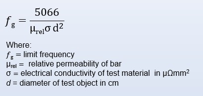
So What is fg?

Here’s the important part: fg is not a test frequency. It’s a mathematical anchor.

It was never intended to be used directly to drive flaw detection. Its real purpose was to let engineers and analysts scale the effects of frequency across different setups.

This allowed for the development of standardized impedance diagrams, which plotted normalized frequency as f/fg.

With these diagrams, inspectors could:

1. Choose the product form (e.g. thin-wall tube, thick-wall tube, rod)

2. Locate an optimal point on the curve (e.g. where the phase is steepest or most sensitive)

3. Multiply the f/fg ratio by the calculated fg to get a real-world test frequency.

Did You Know? The Real Difference Between fg and fc

Most modern textbooks and training materials tweak Förster’s formula by using:

• Wall thickness in millimeters or inches

• Conductivity in %IACS

• Modified constants

When this happens, the correct designation isn’t fg—it’s fc (characteristic frequency).

How Förster Came Up with fg

What makes Förster’s fg so brilliant is that it wasn’t reverse-engineered from data—it was abstracted from physics.

He understood that penetration depth depends on test frequency, material conductivity, and material permeability, and that wall thickness introduces a geometric constraint. But instead of asking, what frequency gives me a certain depth?, he asked:

By formulating fg the way he did, he created a dimensionless ratio—f/fg​—that could be used to scale and interpret impedance behavior, regardless of the material or tube size.

This insight is what enabled the Similarity Law.

The Similarity Law

Förster’s Similarity Law states:

That’s why fg matters—even today. It allows us to:

• Predict signal behavior

• Scale results across materials

• Interpret data from standard curves.

From fg to F90: The Big Shift

Over time, the field moved away from impedance diagrams and scaling exercises. Technicians needed a quicker, simpler way to set up inspections.

That’s where F90 came in—a test frequency that gives about 90° phase separation between near-side and far-side flaws. It’s practical, easy to apply, and more intuitive in field use.

The image below shows one current-day methodology for developing the F90 test frequency for nonferrous tubing exams:

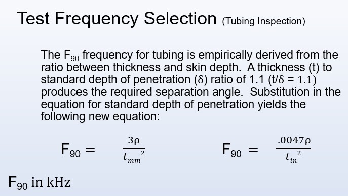
Today, most inspectors choose a test frequency just above and below F90 and fine-tune it from there.

Richard Hochschild: The Unsung Hero

In the 1950s, Richard Hochschild spent six months at Förster’s lab in Reutlingen. When he returned to the U.S., he did a full knowledge transfer, introducing American engineers to:

• The Similarity Law

• Impedance curve analysis

• Limit frequency theory

• Magnetic and nonmagnetic response modeling.

His efforts helped shape the early eddy current standards used by the National Bureau of Standards (now NIST) and industrial labs across the U.S.

✅ Summary: Then and Now

Want to Go Deeper?

Visit eddycurrent.com for:

• Calculators for F90, penetration depth, and more

• Archives of Förster and Hochschild’s historical work

• Slide rules and tools for modern ECT

• The Eddy Current Truths blog series—debunking myths and bridging the old and new.

Final Word

Dr. Förster didn’t just invent formulas. He invented the language of eddy current testing. And thanks to Richard Hochschild, that language spread—evolving from impedance curves and fg to F90 and digital flaw detectors.

So the next time you select a frequency or teach someone how to size a flaw, remember:

And now—you understand what those giants were actually trying to do.