
If you’re scratching your head about permeability in eddy current testing, you’re not alone. Between relative permeability (μᵣ), the permeability of free space (μ₀), and the classic unitless form μ = B/H, it’s easy to get tangled. Let’s unpack why this was once a vital piece of the equation—and why modern eddy current testing often leaves it out entirely.
📚 A Quick Primer on Permeability
In classical electromagnetic theory, permeability (μ) tells us how easily a material can support a magnetic field. It’s a product of:
-
μ = μ₀ × μᵣ
-
μ₀ is the permeability of free space (4π × 10⁻⁷ H/m)
-
μᵣ is the relative permeability of the material.
-
This matters because eddy current behavior—like the standard depth of penetration—is governed by formulas like the Libby/Franklin expression:
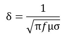
The formula in Figure 1 uses conductivity (σ), and you can see μ is tucked away in the denominator. That’s where the confusion starts.
So Why Use μ at All?
In early eddy current systems, particularly those covered by Libby and Franklin, permeability was essential for precise modeling—especially for ferromagnetic materials. This is because μᵣ can vary widely (e.g., from ~1 for aluminum to 1000+ for steels), dramatically affecting penetration depth, impedance, and signal phase.
For example, in Förster-style testing of cylinders and spheres, permeability is vital in calculating the impedance trajectory on the complex plane. But this comes at a cost: working with SI units like Siemens per meter (S/m) and Henries per meter (H/m) introduces really large and really small numbers—awkward for quick calculations.
Modern Shortcuts: %IACS and μΩ·cm
The 1970’s saw a boom in ECT applications, particularly in the aviation and nuclear industries. Nonferromagnetic materials like aluminum, titanium, and nickel alloys are very common engineering materials that do NOT need to permeability considerations when determining test frequency for standard depth of penetration.
To streamline field use, eddy current practitioners began using derived versions of the earlier formulas, rewritten in user-friendly terms. Instead of working in S/m and H/m, most modern calculations are done with:
-
%IACS (percent of International Annealed Copper Standard) for conductivity, or,
-
μΩ·cm (micro-ohm-centimeters) for resistivity.
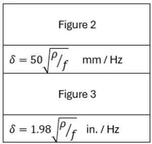
So what if you have the conductivity value expressed in %IACS, but not resistivity in μΩ·cm? No problem! You just convert %IACS to resistivity, and use the formula in Figure 2 or 3. in These units are directly tied to non-ferromagnetic materials, where μᵣ ≈ 1 and can be ignored. The formulas are scaled accordingly so you don’t need to explicitly enter μ at all.
Why? Because for nearly all non-magnetic testing, the permeability is constant and cancels out during unit conversions or gets baked into the constants. These simplified equations provide highly accurate results without the math headache.
Can the Libby/Franklin Formula Be Used for Ferromagnetic Materials? ✅
Yes—but only if you explicitly include μ. The Libby/Franklin formula is general and works for any material as long as you correctly use the full permeability μ = μ₀ × μᵣ. If you forget to include μᵣ for a ferromagnetic sample, your depth calculations could be wildly wrong.
This is one reason early eddy current modeling was so challenging. Effective permeability varies with frequency, material geometry, and even flaw depth, especially in ferromagnetic parts. Tables, correction factors, and complex impedance plane analysis were all used to manage this variability.
💡 Bottom Line
If you’re working with non-ferromagnetic materials like aluminum, copper, titanium, or Inconel, go ahead and use simplified formulas based on %IACS or μΩ·cm. Permeability is essentially 1, and you’re safe to ignore it.
But if you’re analyzing ferromagnetic parts—especially in flaw sizing or magnetic saturation scenarios—then yes, you need to dust off those μ values and prepare for a deeper analysis.